Man Group unlocks massively parallel option pricing with Graphcore IPU

Econometrics models form the backbone of data driven financial organisations. They allow economic phenomena to be modelled with statistical methods, leading to better-informed decision making.  

Man Group, an active investment management firm headquartered in London, relies on option pricing models such as Cox-Ross-Rubinstein to value millions of options every day. Man Group’s quantitative researchers are continuously working to improve the performance of these models to gain a competitive edge, a search which has recently seen them evaluate IPUs, with impressive results. 

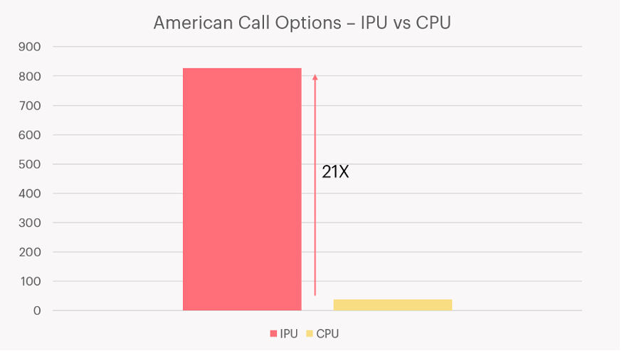
“Option pricing is a critical workload for Man Group, and one that is computationally demanding. The Cox-Ross-Rubinstein method is still a good benchmark for testing this on IPUs. Recent research with Graphcore has demonstrated the massively parallel nature of the IPU, which can price options up to 21x faster than our CPUs,” said Balazs Domonkos, Senior Engineer in Alpha Technology, Man Group. 

CPUs are still frequently chosen over GPUs as the hardware of choice in many financial institutions, due to their flexibility to handle econometrics workloads that cannot be easily vectorised. IPUs provide a good alternative to CPUs, as they can speed up these workloads by providing the same MIMD flexibility as the CPU, while offering much higher flop-rates and processing speed. Three types of hard-to-vectorise workloads that fit into this category are detailed below. 

Conditional termination workloads. These workloads contain loops that continue until a condition is met, or a certain number of iterations have completed which is determined by the inputs. If using batch processing, all samples will have to complete before the batch can be considered complete. Examples include autocallable option pricing models, which can terminate if the autocall event has been triggered. 

Sequential workloads. These can include iterative, loop-based and recursive workloads. In the case of a sequential workload which doesn't need to be run many times, it's not possible to vectorise because the output of the current operation is required as an input to the next. Examples include Hamiltonian Monte Carlo, which iteratively simulates Hamiltonian dynamics. 

Input-dependent routing workloads. These are tree-based models and other forms of models that make use of conditional statements (if-statements). These workloads can be hard to vectorise if the operations performed on each element of the batch diverge. Decision trees with variable depths are a strong example. 

In this blog post, we’ll look at an algorithm known as the Cox-Ross-Rubinstein (CRR) model. CRR is a popular algorithm for options pricing because its flexibility allows it to handle a wide range of conditions, such as the right of an American options holder to exercise the option at any time. We’ll talk through the workings of the CRR model, some of the intricacies that can come with vectorisation, and how you can implement it at scale in production on the IPU. 

Pricing options with the CRR model 

The Cox-Ross-Rubinstein (CRR) model prices an option by considering how the price of the asset could vary over a discrete number of simulated timesteps (n) between the valuation date and the expiration date. The higher the number of simulated timesteps, the more accurate the pricing. 

There are two phases to the model. In phase 1, known as the forward pass, a tree of prices is generated by assuming the price of the underlying asset will either increase or decrease by a specific factor at each simulated timestep, from the current spot price S₀. The factor by which the asset could increase or decrease is calculated as a function of the volatility of the asset and the size of the simulated timesteps.

In phase 2, known as the backward pass, the value of the option is iteratively calculated by moving back through the tree of prices. At each timestep, the value of the option at the previous timepoint is calculated by considering the probability that that underlying would have gone up or down; this is known as the binomial value. 

The binomial parameter p represents the probability of the price going up at any particular simulated timepoint; p is set such that the binomial distribution it represents would simulate Brownian motion of the asset with the measured volatility and assumed discount rate. 

It is important to note that there is a difference in the backward pass of the algorithm when implemented for European options vs American options. This difference capitalises on the flexibility of the CRR algorithm by implementing a condition that reflects the American option holder's ability to exercise the option at any time. 

Side-effects of vectorization 

The power of the CRR algorithm lies in the user's ability to add conditions at any timestep. For pricing American options, a condition is added such that the value of the option cannot be below what could be yielded by exercising the option immediately. 

Despite this condition, it is possible to vectorise the CRR algorithm, both across the height of the tree, and over a batch of options. Such an implementation can be found in Google's tf-quant finance library tf-quant-finance/crr_binomial_tree. The authors vectorise the algorithm across a mixed batch of American and European options. This means the same operations need to be executed, regardless of whether each input in the batch is an American option, or a European option. 

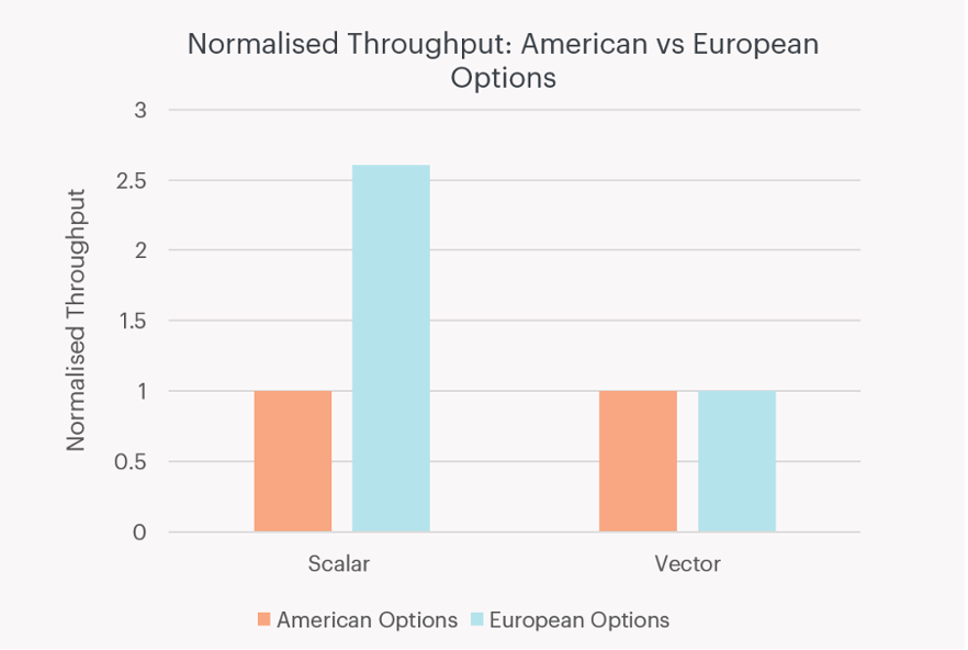
European options should require fewer operations to process than American options because they don’t require calculating whether you could achieve a higher return by immediately exercising the option. However, because this form of vectorisation requires the same operations be executed for pricing American and European options, the throughput is equalised between the two. This is demonstrated in Figure 1. 

For Cox-Ross-Rubinstein, this is remedied without too much difficulty by maintaining two copies of the code, one for European options and one for American options, hence removing the ‘if’ statement. However, for variations of Cox-Ross-Rubinstein and other econometrics models, a fix will not be so simple. 

Another motivation for scalar, rather than vectorised implementations, is that they enforce data locality. When processing a batch with vectorised operations, it is likely that data will be exchanged between compute cores and caches, in preparation for the subsequent operations. This might be avoided with scalar implementations because there are no interdependencies between cores/threads. 

The IPU’s MIMD architecture prices 8832 options in parallel on a single IPU 

MIMD processors, like CPUs and the Graphcore IPU, offer more flexibility than their SIMD counterparts. With the IPU, a thread can execute any instruction regardless of what other threads are doing, while on a SIMD processor each thread must execute the same instruction, hence the need for vectorisation. 

Accommodating input-dependent routing is trivial with scalar operations on an IPU processor. Instead of computing a batch of samples, each sample is distributed to a single thread which is free to execute whichever compute path is needed for that sample. This means if the sample has converged, processing stops, and the thread is returned to the control program. If because of the properties of that sample, the program doesn't require execution of a certain section of code (an if statement), it freely skips it. This fine-grained control is not possible with batch processing. 

Mass option pricing is easily solved in an IPU programming model by treating the hardware as a pool of workers and distributing options to each worker for independent processing. Once a worker has completed processing it returns to the control program and can be dispatched again with another option. This process works similarly on IPUs as it does on CPUs. 

In contrast to the CPU, the IPU is a massively parallel MIMD chip: with 1,472 tiles and 8,832 parallel threads which can operate independently to all other threads. This means, like the CPU, it does not need to rely on vectorised programs to achieve high performance, yet it has 1-2 orders of magnitude more cores than server-grade CPUs available today.  

By mapping a single option to a single processor thread (the IPU has 6 threads per IPU tile), we can price 8832 options in parallel on a single IPU. Below we compare this to a standard server-grade CPU with 24 cores (with 2x hyperthreading giving 48 threads), which prices 48 options in parallel. A throughput comparison between a single MK2 IPU and a single CPU (an Intel Xeon Platinum 8168) can be seen in Figure 2.  

The parallelism offered by the IPU is not the only reason the CRR algorithm runs well on the IPU. The CPU stores the tree of prices in off-chip DRAM, which can be accessed with a read/write speed of roughly 190GB/s, although this is likely improved somewhat through use of the memory hierarchy. The IPU however, explicitly stores the entire tree of prices in its 900MB of in-processor memory (SRAM), which can be accessed with a read/write speed of 47TB/s. 

The CRR algorithm is an example of a workload with input-dependent routing, and we've demonstrated that a popular vectorisation of this workload comes with the downside of running at the speed of the longest possible compute path. 

Conclusion 

CPUs are still chosen as the hardware of choice in many financial institutions due to their flexibility to handle workloads that cannot be easily vectorised. However, the Graphcore IPU can speed up these kinds of workloads by providing the same MIMD flexibility as the CPU, while offering much higher flop-rates and therefore processing speed.