Leveraging the IPU for Molecular Dynamics Simulation

Molecular dynamics uses computers to simulate the movement of molecular and atomic systems. It is a basic method for simulating the microscopic world, and has a wide range of applications in the fields of physics, chemistry, biology, and material science. Molecular dynamics treats each atom in the system as a basic particle that follows Newton’s second law. Given the initial state and time step of the atom, it analyzes the force on the atom (see the calculation in the red box in Figure 1) and establishes the trajectory of the atom.

Molecular dynamics simulation is essential for calculating molecular forces. The traditional method uses the empirical force field to calculate the force of a molecule. In a specific system, it can simulate a system at the scale of tens of billions of atoms, but the precision is limited and it is difficult to handle the simulation of complex systems. In the case of first-principles molecular dynamics based on density functional theory, the calculation precision is high, but the calculation amount is large. The simulation scale is usually limited to hundreds of atoms, within 100 picoseconds. Deep learning provides a new means to analyze the force of atoms. The DeePMD-kit is a typical example, which has both the computational efficiency of the empirical standpoint and the precision of the first principles.

molecular dynamics sim figure 1

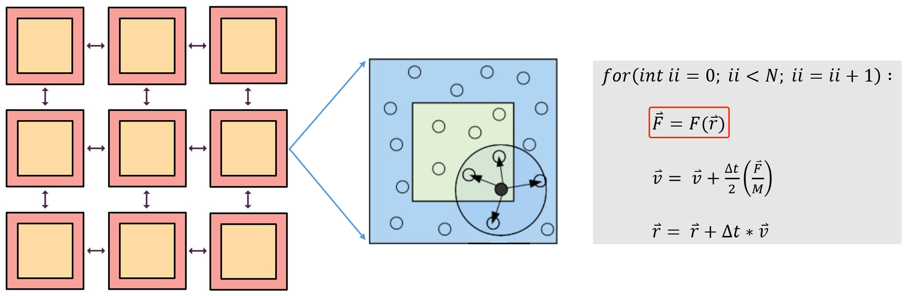
Figure 1: Schematic Diagram of Molecular Dynamics Simulation

Using DeePMD-kit for Force Analysis

molecular dynamics sim figure 2

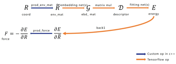
Figure 2: Network Structure

The network structure of force calculation using DeePMD-kit can be seen in Figure 2. Shown from left to right are the input configuration atomic coordinates, environment matrix, embedding matrix, construction of the Descriptor that satisfies symmetry, total energy (E) of the system, and the reverse force calculation. It is worth emphasizing that the generation and force calculation of the environment matrix should be implemented as a TensorFlow Custom Operator, and the remainder uses TensorFlow’s native Operator. We will now briefly introduce the functions of each part.

1. Input configuration

Taking coordinate Coord as an example, the typical MD (Molecular Dynamics) input configuration contains information such as atom type in addition to atomic coordinates (see Table 1 for details).

2. Environment matrix

The environment matrix is usually constructed according to certain rules. For a large system, the system needs to be rasterized into several smaller systems (see the orange squares in Figure 1). In the smaller systems, it is constructed according to the truncation radius (the radius of the circle in Figure 1) and other parameters, and with the central atom in the viewpoint circle, neighbour atoms are selected to construct the environment matrix of the system. It can be seen from Formula 1 and Formula 2 that the environment matrix itself satisfies translation invariance.

Formula 1

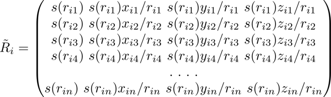
Formula 2

3. Embedding matrix

Embedding matrix is the most primitive feature. The embedding net (see Figure 2) contains trainable parameters, which can construct suitable representations for the relationship between different types of central atoms and neighbours, which is very important for neural network training.

4. Construction of the Descriptor

This step is mainly to add rotation and displacement invariance to the constructed neural network model, which can improve the adaptability of the model so that the model can still accurately predict the energy when the atom is rotated and displaced. This also reduces the dependence on the training set to a degree.

5. Fitting of system energy E

In this step, the energy of the entire system is calculated by inputting the Descriptor into the neural network constructed based on Multi-Layer Perceptron (MLP). In training, the energy of the entire system is usually calculated using first-principles and other high-precision methods.

6. Force analysis

By calculating the derivative of the total energy E against the position, the force of each atom can be obtained. Therefore, the force analysis part of the calculation includes a neural network inversion, which will lead to a higher memory usage. At the same time, the environment matrix uses a Tensorflow Custom Operator to realize the derivation against the position.

Leveraging the IPU for Water Molecule Simulation

When performing water molecule simulation on the IPU, we use a model in SavedModel format. In order to run the model on IPU, we did the following:

Implemented and optimized the TensorFlow Custom Operator on IPU
Set the device attribute of the model to IPU

1. Custom Operator

EnvMat is the environment matrix mentioned above. During processing, we have to calculate the similarity of neighbour atoms of each central atom, then sort, and select the top K neighbour atoms of each central atom, and then substitute it into the formula for calculation. So, this Op's bottleneck is not defined as the calculation part, but the sorting part. In the actual implementation, efficient sorting is finally realized through the combination of QuickSort+InsertSort.

Force and Virial Force, according to the forward result of the network, obtain the partial derivative of x. These two Ops involve the problem of global memory access. Taking into account the limitations of IPU, it is impossible to put all the atomic data on one tile. Therefore, we need to split the global data into N pieces, and then reduce sum on N pieces of data, and finally obtain a complete set of data. Although this can ensure the memory of the IPU is no longer limited, it obviously limits the use of the IPU's computing power, so we need to find a better solution.

2. Set the device attributes of the model

In TensorFlow SavedModel format model, each operation corresponds to a node. By setting different device attributes for different nodes, we can set the execution device of the operation. We edit the device attribute of the node to IPU and put the operation on the IPU for execution.

3. Simulating water molecules on the IPU

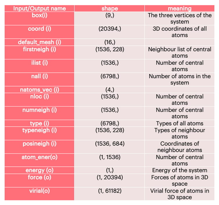
The detailed input and output information of the water molecule model is shown in Table 1. In addition to Coord, it also includes the neighbour information of the central atom, including coordinates and atom types. We construct the environment matrix of each central atom according to the information of firstneigh, typeneigh, and posineigh.

Table 1: Model Input and Output Information

After completing the Custom Operator and setting the device properties, we can finally achieve performance similar to V100 on a system of 1536 central atoms.

4. Memory optimisation

We conducted an in-depth analysis of the water molecule simulation. Since the model itself has a backward process, we need to store some forward calculation results with a total size of about 300MB. This part of the memory overhead can be alleviated by recomputation, enabling us to simulate a larger system.

Summary

We have successfully performed water molecule simulation on the IPU, with the performance achieved on small systems essentially matching V100 performance. Future work will focus on simulating large systems.